This one is a short one and I don't know who its for. Wikipedia talks about an adversarial bandit algorithm that would work well for something I'm working on:

An example often considered for adversarial bandits is the iterated prisoner's dilemma. In this example, each adversary has two arms to pull. They can either Deny or Confess. Standard stochastic bandit algorithms don't work very well with these iterations. For example, if the opponent cooperates in the first 100 rounds, defects for the next 200, then cooperate[sic] in the following 300, etc. Then algorithms such as UCB won't be able to react very quickly to these changes. This is because after a certain point sub-optimal arms are rarely pulled to limit exploration and focus on exploitation. When the environment changes the algorithm is unable to adapt or may not even detect the change. 
  

Ok, lets try it out. Wikipedia gives the algorithm, but to make this blog look sick I'll repost it here. The idea is to pick the correct "arm" at any given time point. So, if the adversary confesses 100 times in a row, we should choose the arm that maximizes our gain, if our adversary then switches tacticts, we should rethink our strategy.

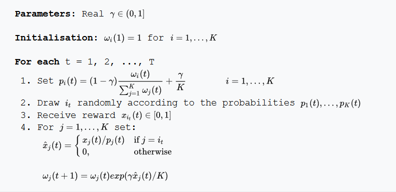
I'll work on syntax highlighting later, but the code is below. The biggest thing to note is that the most recent "arm" that is chosen gets exponentiated, if it is the correct arm.

distr <- function(weights, gamma){
  sum <- sum(weights)
  (1.0 - gamma) * (weights / sum) + (gamma / length(weights))
}

exp3 <- function(num_choices, winners, gamma, N){
  weights <- rep(1, num_choices)
  choices <- rep(NA, num_choices)
  for(i in 1:N){
    prob_dist <- distr(weights, gamma)
    choice <- sample(1:num_choices, 1, prob = prob_dist)
    choices[i] <- choice
    reward <- ifelse(winners[i] == choice, 1, 0)
    estimated_reward <- 1.0 * reward / prob_dist[choice]
    weights[choice] <- weights[choice] * exp(estimated_reward * gamma / num_choices)
  }
  return(list(choices = choices, weights = weights, prob = prob_dist))
}

Awesome- we can call it with the code below. We create 500 trials, where the first 100 are most likely to be choice 2, followed by 200 choices of most likely 1, and finally 300 choices of most likely 2. Overall, we should have around ~2/3s of our trials be choice 2 while 1/3 are choice 1. (R uses 1-based indexing, get over it). This is exactly what Wikipedia says this algorithm will excel at.

winners <- c(rbinom(100, 1, .9), rbinom(200, 1, .1), rbinom(300, 1, .9)) + 1

N <- length(winners)
num_choices <- 2
gamma <- .05

c <- exp3(num_choices, winners, gamma, N)

For this type of problem the metric most people care about is regret (which is defined on the wiki page), but for our purposes I only care about how many times we correctly chose the winner. The result of my simulations showed 53% success. To me, instinctively this doesn't feel great. Looking at the internals of the state show that at some point, the exponentiated weights are too big to surpass. After the first 100 trials the weights are 4.75 and 7,096,892.22, respectively. It then takes 100 more trials for the weights to even out. Let's compare this vs a greedy strategy.

epsilon <- function(num_choices, winners, epsilon, N){
  wins <- rep(1, num_choices)
  trials <- rep(2, num_choices)
  choices <- rep(NA, num_choices)
  for (i in 1:N){
    prop <- wins / trials
    conf_prop <- prop - 1.96 * (sqrt(prop * (1- prop)/ n))
    if(runif(1, 0, 1) > epsilon){
      choice <- which.max(conf_prop)
    }
    else{
      choice <- sample(1:num_choices, 1)
    }
    trials[choice] <- trials[choice] + 1
    reward <- ifelse(winners[i] == choice, 1, 0)
    wins[choice] <- wins[choice] + 1
    choices[i] <- choice
  }
  return(list(choices = choices, success = (wins / trials)))
}

The big difference here is that the most recent winner isn't exponentiated. Also- instead of sampling the winners via their likelihood, we use a parameter called epsilon. If rand > epislon we only choose the best arm. How does it do? My simulations show ~37% success. Significantly worse that the adversarial algorithm. Still, I can't help but think that using sliding time scale, or even some form of bayesian changepoint detection would outperform either of these methods on this toy problem. Maybe next blog?